Spectrum visualization
The quickstart briefly introduced the spectrum_utils plotting functionality.
Often, nice spectrum graphics can be created with only a single line of code; it’s as easy as using spectrum_utils.plot.spectrum(...) to visualize a single spectrum.
Here we will briefly describe some advanced functionality to customize your spectrum plots.
Some of the arguments that can be provided to spectrum_utils.plot.spectrum(...) are:
color_ions: Boolean flag indicating whether the annotated peaks should be colored.annot_fmt: A function that converts aFragmentAnnotationto a label to annotate the corresponding peak (see below).annot_kws: A dictionary with options to customize peak label texts. See thematplotlib.text.Textdocumentation for available options.grid: Enable/disable the grid.
See the API reference for full details on how to use these settings.
Peak annotations
By default, singly-charged b and y peptide fragment ions are annotated with a label in the spectrum plots.
To avoid overcrowding the spectrum plots, other peaks will be highlighted in the matching color, but will not receive an annotation label.
However, which peaks to annotate and the format of the label can be fully customized by providing a callable that implements your desired behavior to annot_fmt.
Here we will show example code that can guide you in implementing your custom peak labeling functionality. As mentioned previously, the default implementation labels singly-charged b and y peptide ions that have not undergone a neutral loss (slightly adapted for conciseness):
def annotate_ion_type(annotation, ion_types="by"):
    if (
        annotation.ion_type[0] in ion_types
        and annotation.neutral_loss is None
        and annotation.isotope == 0
        and annotation.charge == 1
    ):
        return annotation.ion_type
    else:
        return ""
To annotate additional ion types, you can reuse the default implementation in combination with functools.partial:
import functools
import spectrum_utils.plot

spectrum_utils.plot.spectrum(..., annot_fmt=functools.partial(ion_types="abyIm"))
Peak labels that contain full information according to the PSI peak interpretation specification can be achieved by using the str function: spectrum_utils.plot.spectrum(..., annot_fmt=str).
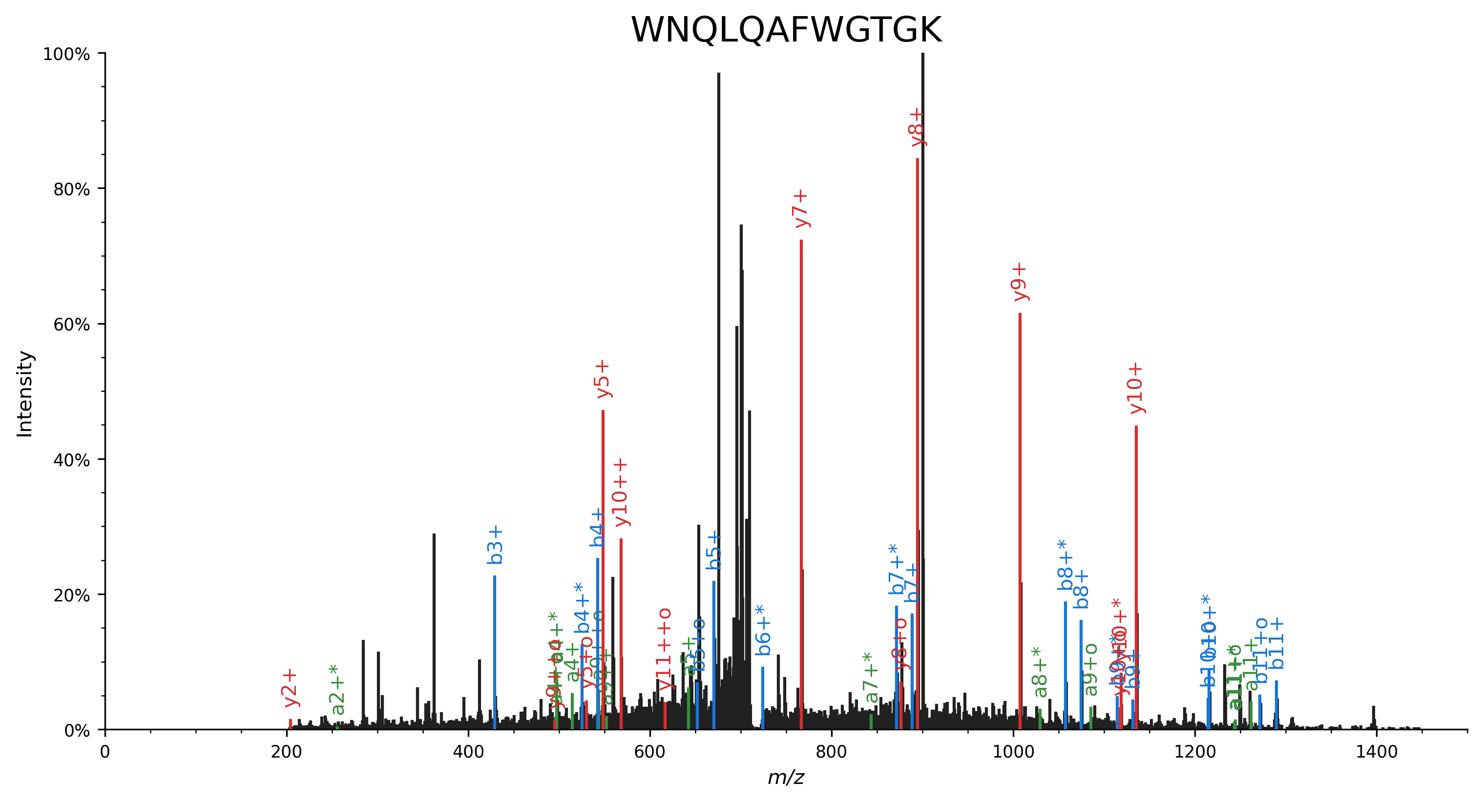
Finally, we’ll show an example of custom peak labeling functionality that indicates the charge state by repeated + symbols, neutral loss of ammonia by the * symbol, and neutral loss of water by the o symbol. This behavior is similar to the Lorikeet spectrum viewer.
import matplotlib.pyplot as plt
import spectrum_utils.plot as sup
import spectrum_utils.spectrum as sus


def annotate_ion_type(annotation, ion_types="aby"):
    if annotation.ion_type[0] in ion_types:
        if abs(annotation.isotope) == 1:
            iso = "+i" if annotation.isotope > 0 else "-i"
        elif annotation.isotope != 0:
            iso = f"{annotation.isotope:+}i"
        else:
            iso = ""
        nl = {"-NH3": "*", "-H2O": "o"}.get(annotation.neutral_loss, "")
        return f"{annotation.ion_type}{iso}{'+' * annotation.charge}{nl}"
    else:
        return ""


usi = "mzspec:PXD014834:TCGA-AA-3518-01A-11_W_VU_20120915_A0218_3F_R_FR01:scan:8370"
peptide = "WNQLQAFWGTGK"
spectrum = sus.MsmsSpectrum.from_usi(usi)
spectrum.annotate_proforma(
    peptide,
    fragment_tol_mass=0.05,
    fragment_tol_mode="Da",
    ion_types="aby",
    max_ion_charge=2,
    neutral_losses={"NH3": -17.026549, "H2O": -18.010565},
)

fig, ax = plt.subplots(figsize=(12, 6))
sup.spectrum(spectrum, annot_fmt=annotate_ion_type, grid=False, ax=ax)
ax.set_title(peptide, fontdict={"fontsize": "xx-large"})
ax.spines["right"].set_visible(False)
ax.spines["top"].set_visible(False)
plt.savefig("annot_fmt.png", dpi=300, bbox_inches="tight", transparent=True)
plt.close()
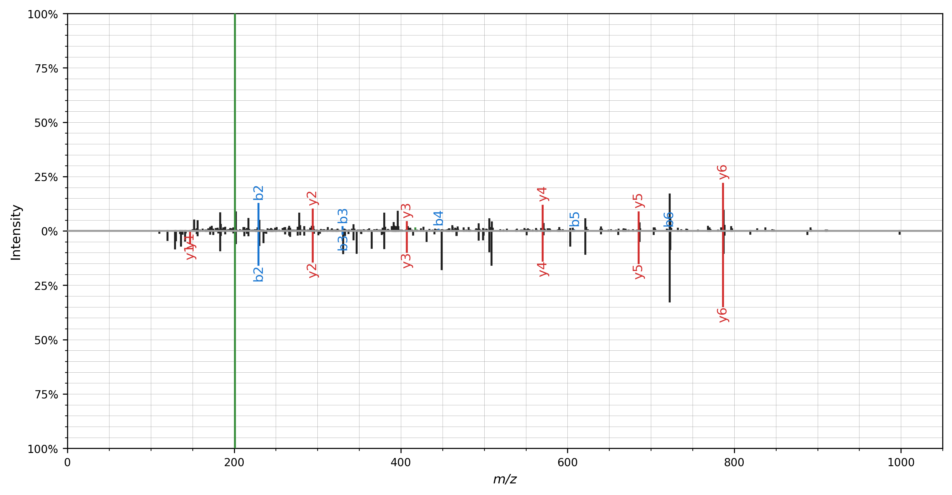
Mirror plot
A mirror plot can be used to visualize matching spectra, for example, to plot identifications from spectral library searching.
Again, only a single line of code is required to do the actual plotting: spectrum_utils.plot.mirror(...)
import matplotlib.pyplot as plt
import spectrum_utils.plot as sup
import spectrum_utils.spectrum as sus


peptide = "DLTDYLM[Oxidation]K"
usi_top = "mzspec:MSV000079960:DY_HS_Exp7-Ad1:scan:30372"
spectrum_top = sus.MsmsSpectrum.from_usi(usi_top)
spectrum_top.annotate_proforma(peptide, 0.5, "Da", ion_types="aby")
usi_bottom = "mzspec:MSV000080679:j11962_C1orf144:scan:10671"
spectrum_bottom = sus.MsmsSpectrum.from_usi(usi_bottom)
spectrum_bottom.annotate_proforma(peptide, 0.5, "Da", ion_types="aby")

fig, ax = plt.subplots(figsize=(12, 6))
sup.mirror(spectrum_top, spectrum_bottom, ax=ax)
plt.savefig("mirror.png", dpi=300, bbox_inches="tight", transparent=True)
plt.close()
All of the advanced plotting arguments described above can be provided for the mirror plot as well using the spectrum_kws argument.
Mass error plot
The difference between the observed and the theoretical mass of annotated fragment ions can be visualized in a mass error plot. In these bubble plots, the size of the bubbles corresponds to the intensity of the fragment ions, the x-axis shows the observed m/z, and the y-axis shows the mass error either ppm or in Dalton. Use spectrum_utils.plot.mass_errors(...) to plot mass errors:
import matplotlib.pyplot as plt
import spectrum_utils.plot as sup
import spectrum_utils.spectrum as sus

usi = "mzspec:PXD022531:j12541_C5orf38:scan:12368"
peptide = "VAATLEILTLK/2"
spectrum = sus.MsmsSpectrum.from_usi(usi)
spectrum.annotate_proforma(
    peptide,
    fragment_tol_mass=0.05,
    fragment_tol_mode="Da",
    ion_types="aby",
    max_ion_charge=2,
    neutral_losses={"NH3": -17.026549, "H2O": -18.010565},
)

fig, ax = plt.subplots(figsize=(10.5, 3))
sup.mass_errors(spectrum, plot_unknown=False, ax=ax)
plt.savefig("mass_errors.png", dpi=300, bbox_inches="tight", transparent=True)
plt.close()
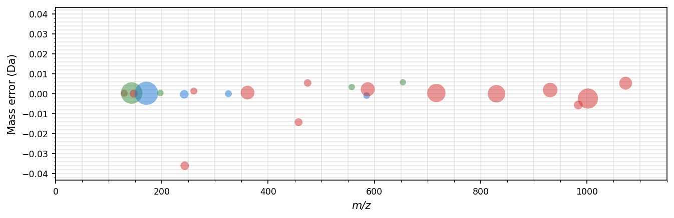
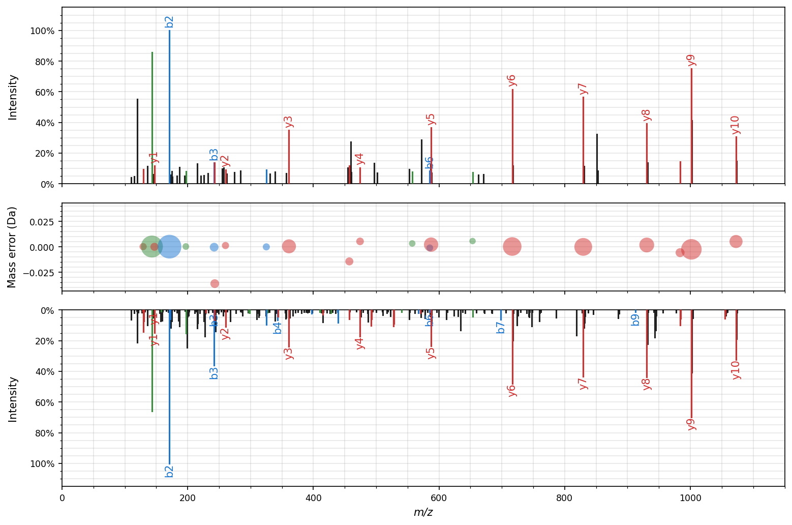
Figure-level facet plot
The figure-level spectrum_utils.plot.facet function combines the spectrum_utils.plot.mirror and spectrum_utils.plot.mass_errors functionality:
import matplotlib.pyplot as plt
import spectrum_utils.plot as sup
import spectrum_utils.spectrum as sus

peptide = "VAATLEILTLK/2"
annotation_settings = {
    "fragment_tol_mass": 0.05,
    "fragment_tol_mode": "Da",
    "ion_types": "aby",
    "max_ion_charge": 2,
    "neutral_losses": {"NH3": -17.026549, "H2O": -18.010565},
}

usi_top = "mzspec:PXD022531:j12541_C5orf38:scan:12368"
spectrum_top = sus.MsmsSpectrum.from_usi(usi_top)
spectrum_top.annotate_proforma(peptide, **annotation_settings)

usi_bottom = "mzspec:PXD022531:b11156_PRAMEF17:scan:22140"
spectrum_bottom = sus.MsmsSpectrum.from_usi(usi_bottom)
spectrum_bottom.annotate_proforma(peptide, **annotation_settings)

fig = sup.facet(
    spec_top=spectrum_top,
    spec_mass_errors=spectrum_top,
    spec_bottom=spectrum_bottom,
    mass_errors_kws={"plot_unknown": False},
    height=7,
    width=10.5,
)
plt.savefig("facet.png", dpi=300, bbox_inches="tight", transparent=True)
plt.close()
Interactive plotting
Besides the standard plotting functionality in spectrum_utils.plot, spectrum_utils also contains interactive plotting functionality in spectrum_utils.iplot.
iplot is a drop-in replacement for plot; only the import statement needs to be changed to produce interactive plots.
Interactive plot of an individual spectrum:
import spectrum_utils.iplot as sup
import spectrum_utils.spectrum as sus


usi = "mzspec:PXD004732:01650b_BC2-TUM_first_pool_53_01_01-3xHCD-1h-R2:scan:41840"
spectrum = sus.MsmsSpectrum.from_usi(usi)
spectrum.annotate_proforma("WNQLQAFWGTGK", 10, "ppm", ion_types="aby")

chart = sup.spectrum(spectrum)
chart.properties(width=640, height=400).save("iplot_spectrum.json")
Interactive mirror plot of two spectra:
import spectrum_utils.iplot as sup
import spectrum_utils.spectrum as sus


peptide = "DLTDYLM[Oxidation]K"
usi_top = "mzspec:MSV000079960:DY_HS_Exp7-Ad1:scan:30372"
spectrum_top = sus.MsmsSpectrum.from_usi(usi_top)
spectrum_top.annotate_proforma(peptide, 0.5, "Da", ion_types="aby")
usi_bottom = "mzspec:MSV000080679:j11962_C1orf144:scan:10671"
spectrum_bottom = sus.MsmsSpectrum.from_usi(usi_bottom)
spectrum_bottom.annotate_proforma(peptide, 0.5, "Da", ion_types="aby")

chart = sup.mirror(spectrum_top, spectrum_bottom)
chart.properties(width=640, height=400).save("iplot_mirror.json")
For more information on how to manipulate these interactive plots, see the Vega-Altair documentation.
Interactive plots can be saved as html files or other output formats, and can be embedded as JSON into web pages using Vega-Embed.
Miscellaneous
Peak colors
By default, peaks are colored based on their ion type as follows:
a peptide fragments (
"a")b peptide fragments (
"b")c peptide fragments (
"c")x peptide fragments (
"x")y peptide fragments (
"y")z peptide fragments (
"z")internal fragment ions (
"m")immonium ions (
"I")intact precursor ions (
"p")unknown and unannotated ions
To change these colors, overwrite values in the spectrum_utils.plot.colors dictionary with your preferred colors:
import spectrum_utils.plot as sup


sup.colors["y"] = "#FF1493"